Similarity Search - opportunity for PMEM
At a high level, computing solves problems. These problems, even though different and individual, are sometimes somehow related. A new algorithmic challenge can usually be solved by bringing it down to a well-defined problem with an existing solution. Today, we will be talking about one of such universal solutions - similarity search, which has found its application in various areas of life, from search engines that tell us what we want to find, through recommendation engines that tell us what to watch, where to eat and what to buy, all the way to data science that provides valuable input to business decisions.
Similarity Search - what is it?
Vector similarity search is a class of problems in which, given a query vector, a set of vectors and a metric (instruction how to measure distance), we need to retrieve the most similar vector to the query vector from the set. By similar, I mean - the one that has the shortest distance to the query vector in the given metrics.
Why do we need it?
We’ve already defined what the class of problems is and what the areas of application are, but how do they relate to each other? The answer is, we can use vectors to represent things. A vector can be used to represent someone’s social network profile, a word, an item in an online shop, an online article, a photo or virtually anything else we can think of. Also, the distance between two vectors, in general case, is not constrained to some particular metrics, e.g. euclidean (the one we use to compute distance in the real world). If we come up with an idea on how to measure a distance between a donkey and the sound of scratching a blackboard, it’s good enough for the algorithm. And what about finding similar things? We often look for similar items in online shops, similar movies to the ones we watched, search for similar food… Nonetheless, it would be a huge understatement to say that similarity search can only be applied to areas where we directly search for similar things; it constitutes a building block for many other mathematical problems, with many more real-life applications.
I think it’s clearly visible that this solution is important and has a vast array of different applications.
Computational complexity at scale
OK, so what’s the big deal? Every computer science student knows how to code an efficient solution to this problem in a couple of minutes. We can just check all items in the given set and select the best fit, in linear time per query. The thing is, linear time is sometimes not enough. What if a single vector has a couple of kilobytes, the set of vectors takes up several terabytes and our system requires to query thousands of items per second? This is not as abstract as it may seem. Large e-commerce stores, search engines that look for similar images or large-scale recommendation systems might not be far away from these figures.
Approximate Nearest Neighbor
It turns out that, if we sacrifice accuracy, we can get the complexity down to O(log(n)). Today, we will focus on one particular algorithm: Hierarchical Navigable Small World (HNSW) and on how we can leverage PMEM to achieve better TCO (Total Cost of Ownership) of a server machine that runs this algorithm.
Hierarchical Navigable Small World - concept behind the algorithm
Let’s show the concept as an allegory to a database where, in order to quickly retrieve elements, data structures such as indexes are used. Imagine that we have an unsorted table of entries and we want to quickly retrieve some elements, in logarithmic time. We can do that by creating a (sorted by the column of interest, binary tree-based) set of pointers to rows; now, whenever we have a query to process, we can just retrieve the corresponding element(s) from the set, which should take O(log(N)) time (or O(log(N)+M) if we want to retrieve M consecutive elements). Can we implement such index in our case? The problem is, we can really only sort scalars this way - basically, a reduced 1D vector. We can, however, create a graph-based helper structure that can, depending on its size, retrieve the most similar vector with some precision-recall/latency trade-off.
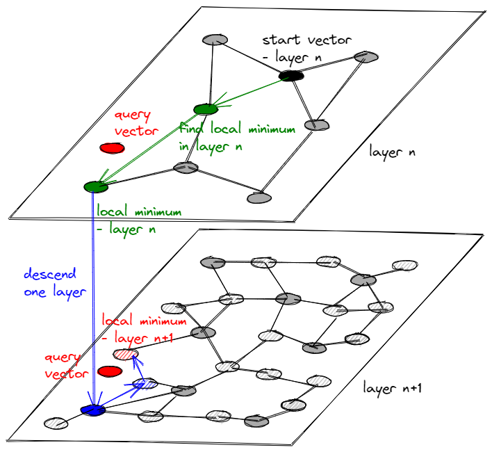
First of all, let’s try to spatially imagine the data structure. We can describe the data structure as a multi-layered graph, where each layer lies on a plane. Each node on a plane is connected to N closest nodes and each node in a layer is also a node in a lower layer; every lower layer contains more elements than the layer above, preferably using some ratio (e.g. +50%).

How do we traverse such a data structure? Given a query vector V, we:
- Start at a node in the top layer
- Find a local minimum in a greedy way within the current layer and select it
- Are we in the lowest layer? If not, descend one layer down and jump to point 2.
- Congratulations, we have retrieved the nearest neighbor of V! Or have we?
For a short recap, how to find a local minimum on a single layer:
- Check distance to all directly connected nodes in the same layer
- Find the closest node
- Is this node closer to V than our current node? If yes, select that node and jump to point 2
- We have reached a local minimum, search on this layer is done
As I’ve already mentioned, this is an approximate solution - the node that we found using this greedy approach might not be the nearest neighbor but, oftentimes, this is not really that much of a problem.
There are other questions that might appear - what about the graph structure? How many layers should it have? How many nodes should each layer contain? They are very important, as the exact values will impact the trade-off between performance and accuracy, but the topic of graph optimization lies outside of the scope of this article.
Why is Optane a great fit?
We now know how to retrieve the vectors of interest in logarithmic time, so wouldn’t this algorithm work well, even without Optane? The answer is, it would. The original paper does not mention storage media other than “RAM”, but we can use Optane products to lower the cost.
As we’ve already mentioned, we have a layered graph that we have to traverse. We can make a few observations:
- each layer would have nodes with different access frequency,
- the access frequency in a layer should be uniform, given that we uniformly query all vectors,
- given two layers - top and bottom, the nodes in the top one would have higher access frequency than the ones below.

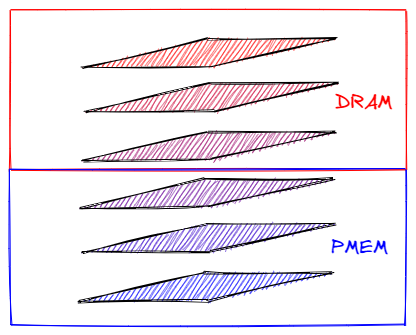
In short, all the nodes are already grouped by their access frequency. As you might have guessed, storing the not-so-frequently accessed nodes on a cheaper medium with higher latency would not hurt the performance that much, while allocating just a little bit of the most performant memory to the top layers can give us a significant performance boost. This is where the Optane technology comes in - a byte-addressable, sweet spot between destined for the top layers DRAM and slow SSD-based storage.
Moreover, from the developer point of view, the accesses to nodes are virtually random; in such case, it’s not just the higher bandwidth and lower latency that gives us an edge over SSDs, but also the byte-addressability and smaller overhead of fetching small chunks of memory.
Another great advantage of this solution is the consistency of lookup time - each lookup needs to traverse through both DRAM and PMEM in rather consistent proportions, which is much better than having random buffered/unbuffered SSD accesses.
Using Optane hardware is the approach taken by the University of California, Merced and Microsoft Research in HM-ANN: Efficient Billion-Point Nearest Neighbor Search on Heterogeneous Memory. In that particular case, only the elements stored entirely in the lowest layer were allocated to PMEM.
What about other storage types, such as SSD and HDD? The common practice is to either perform all calculations in DRAM which, if possible, is costly or to use SSDs, which incurs some performance penalty. In short yes, SSDs can be used for scaling similarity search algorithms and some of the solutions are among state-of-the-art. In fact, many algorithms destined for SSDs can be adapted for PMEM in order to take advantage of the lower latency. On the other hand, given that HDDs have to physically move a mechanical part for each random access and the data access pattern - random reads of very small chunks of memory, HDDs perform especially poor.
Nonetheless, a question arises - how many layers should be placed on DRAM, how many on PMEM? Again - this should be configured accordingly to the SLA that has to be met and can be considered a part of graph optimization, which is a topic for another article.
Is HNSW the state-of-the-art solution?
The algorithm was used to present a concept behind graph-based similarity search and the opportunities for Optane that come with it, so describing state-of-the-art solution was not the goal of this article. The research in this area is still in progress, especially given a variety of hardware that can be leveraged to increase throughput or lower TCO.
Also, the topic of this article was not to present a particular PMEM-enabled implementation of HNSW or any other algorithm, but rather to show how the properties of PMEM can be leveraged. We will be happy to describe a particular implementation once we have an official, open-source library destined for PMEM in particular.
What is noteworthy, HNSW is not the only algorithm adapted to work with heterogeneous memory. Other algorithms, such as DiskANN or SPANN, take slightly different approaches to the problem and leverage heterogeneity differently. The former compresses vectors and keeps them in DRAM, while the graph and full vectors are stored in a slow memory tier. The latter clusters vectors and holds centroids in DRAM and uses SSD storage to keep full posting lists. It shows that heterogeneous memory, in general, is the key to optimizing costs in similarity search.
Billion-Scale Approximate Nearest Neighbor Search Challenge
As similarity search is a crucial area of research for numerous practical applications, Billion-Scale Approximate Nearest Neighbor Search Challenge was organized as a part of NeurIPS 2021 Competition Track. Intel, with its OptaNNE GraphANN solution, was announced as a co-winner of the track 3 of the competition. The solution encompassed both, graph-based software and PMEM hardware. Intel’s solution performed especially well in the TCO category - total cost to horizontally replicate a system to serve 100 000 requests per second, with the cost being almost 20 times lower than that of the second-best solution, CUANNS IVFPQ, for the BIGANN and DEEP data sets (DEEP: 16.1 vs 303.9, BIGANN: 15.4 vs 304.2). GraphANN is an adaptation of DiskANN to PMEM. The competition and its results are described in more details on the official Intel website.
| Algorithm | DEEP | BIGANN | MS Turing | MS SpaceV | Text-to-image | SSN++ |
|---|---|---|---|---|---|---|
| baseline | 545.6 | 737.9 | 853.9 | 735.9 | 1272.7 | 428.1 |
| OptaNNE GraphANN | 16.1 | 15.4 | 16.3 | 16.4 | 103.6 | - |
| CUANNS IVFPQ | 303.9 | 304.2 | 153.2 | 153.2 | 916.8 | - |
| CUANNS MultiGPU | 569.1 | 569.2 | 286.9 | 398.2 | 1213.8 | 629.4 |
Total cost to horizontally replicate a system to serve 100 000 queries per second
Please consult the official results for the exact figures for all categories and data sets, as only selected results that showed the benefits of PMEM were presented here.
Is the OptaNNE GraphANN library open-source?
As of June 13, 2022, it is not. We will keep you informed about any possible updates.

